From Correlation to Causation through stories and math

Correlation and causation are two concepts that people often mixup in their minds. I must admit that I myself have been guilty about this, and it unlikely that I would ever entirely grow out of it as it is wired deeply into our psychology. Let me use this article to briefly emphasise what the concepts of correlation and causation means, some interesting stories that have emerged from people misunderstanding these concepts and an algorithm that attempts to find causal relationship using correlation information.

Here is a story that I heard a professor of mine, Prof. Dr. Ernst-Jan Camiel Wit, tell us during a lecture. There was a school that was involved in a study to see if providing free mid-day meals to students, which they could choose to be subscribed to this or not. At the end of the study, both the students who subscribed to it and did not where tested for different health indicators. It was observed that the students who chose to have meals from the programme had poorer health indicators.

In this example, one could be tempted to conclude that the mid-day meal programme may have caused this issue. Some may believe that the people higher up in the chain may have been corrupt and stole from the pot, whereas some others may believe that the funds provided were not sufficient. But the actual cause of this was that most students who did not choose to enrol in the programme believed that students who are less fortunate should benefit from this programme more, and hence most of the students who enrolled in the programme were otherwise poor. In other words, students who enrolled in the programme were not likely to have other sources of food, and they may have relied solely on the programme, whereas the students who did not enroll had plenty of other options to provide themselves with the required nutrients.

Here is another story from somewhere in North America in the eighteenth or nineteenth century. There were certain female people who lived in towns and cities with a certain coloured cat. At some point, there were certain diseases that affected everyone except these women, then people assumed that they were doing some dark magic to cause this, called them witches and often hunted them down. Sighting their cat was considered a bad omen as well. Now we know that the diseases were actually spread by rats and these women were safe because their cats ate the rats and prevented further spread of diseases to their owners.

There are several stories like such where people tend to associate correlation with causation. Indeed, if Event A causes Event B, the correlation between Event A and Event B would be high. However, if the correlation between Event C and Event B are high, that does not necessarily mean that Event C causes event B or viseversa.

There are also interesting scenarios where the direction of causality are misunderstood. Generally when we observe events such as the road being wet and rain falling, we do not assume that the wet road caused the rain to fall. However, I recently came to read an article stating that accummulation of cholestrol in the arteries are to ameliorate some damagest with the arteries; that is, they do not cause the issues with the arteries, rather they attempt to solve the issues with the arteries. Please do note that I am not a medical professional, nor a builogist; I simply attempt to make myself informed as I love the process, and it is possible that I may miss a thing or two while at it.

Now, it is easy to collect data and observe correlations between different variables. My favourite way of doing this is using a method called partial correlation. It measures the degree of association between two random variables, with the effect of a set of controlling random variables removed. If X represents a column that states how much it rained and Y represents a column that states how much rise in the lake nearby was observed, then the partial correlation is defined as:

\[P_{xy} = \frac{Cov(X,Y)}{\sqrt{Cov(X,X) Cov(Y,Y)}} \]

Note that Cov(X,Y) means the covariance between X and Y. If we have N rows of data for X and Y, then this is defined as:

\[ Cov(X,Y) = \frac{\sum_{i=1}^{N} (X_i - \overline{X}) (Y_i - \overline{Y})}{N} \]

where X_i and Y_i corresponds to the data in the i^th row, and X and Y corresponds the mean values of X and Y, respectively.

The value of partial correlation can be between -1 and 1. A positive value for partial correlation means that if one increases the other also increases, whereas a negative value of partial correlation means that if one increases the other decreases. As partial correlation value gets closer to zero, it means that the two are not really correlated any anywhich way.

This can be applied to large chunks of data with several rows and columns. People sometimes create graphs to show what is correlated to what, which is a very lovely way to visualize. For example, the following is a plot that I indicating an absolute partial correlation value greater than a certain threshold between stock prices for different stocks in the time interval between January 2017 and June 2022.

As we have already discussed, arriving at causal direction between different correlations is hard. Generally, we need to extensively study and evaluate to know what exactly is happening to know what the causal direction is. However, there is an algorithm I am familiar with that attempts to find the direction of causality, called PC Algorithm.

Named after it’s authors Peter Spirtes and Clark Glymour, PC Algorithm is a statistical causal analysis technique used to infer cause and effect from data based on conditional independence. The algorithm starts with a complete connected graph, then remove some of the edges by considering the conditional independence between different nodes to form a skeleton graph that is undirected, and, finally orient the edges based on certain orientation rules to form a partially directed graph. Note that there are cases where PC Algorithm wouldn’t be able to determine the direction of causality and hence the final output is partially directed.

The following are the steps followed by PC algorithm to discover causal connections.

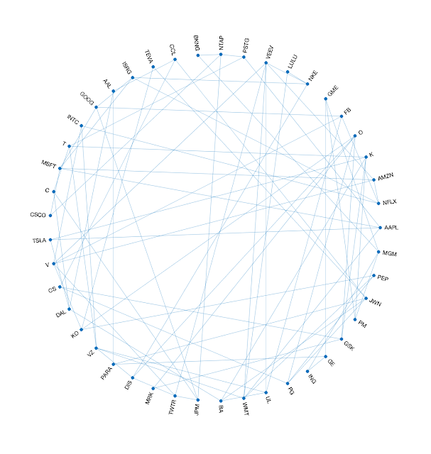
1. Create an undirected graph that represents conditional dependence or correlation between different fields (like the graph you saw earlier).
2. Apply causal orientation rules, which are:
1. Collider rule
   If nodes X_i and X_j are connected to X_k, and X_i is independent of X_j, then the direction of causality would point from X_i to X_k and X_j to X_k.
2. Consistency rules
   These include avoiding cycles, avoiding new colliders and other inconsistencies that we can logically determine. Avoiding new collider means that if nodes X_i and X_j are connected to X_k and X_l, then we do not create a new collider with X_l. Rather, we would connect X_i to X_k, X_j to X_k, and X_k to X_l.

Indeed, there are modified versions of PC Algorithm with more advanced rules. Also, it is to be noted that PC Algorithm does not always lead to the creation of Directed Acyclic Graph; as it is possible that the algorithm may not be able to find the causal direction between certain nodes, the overall graph can be Partially Directed Acyclic Graph.

The following is the result of applying PC Algorithm to the graph that was shown earlier. We can visualize how prices of certain stocks affect the prices of certain other stocks.

Should you wish to try this on your own, there is a PC Algorithm package for R language, which you can download from the link below.

https://cran.r-project.org/web/packages/pcalg/index.html

It must be noted that PC Algorithm is just a tool that gives you a reasonable idea for the direction of causality, and it need not always give you the right direction. While performing the analysis, people sometimes use their intuition and knowledge to provide initial information on the direction of causality for certain nodes.